Welcome to adobo’s documentation!

What adobo is

adobo is an analysis framework for single cell RNA sequencing data (scRNA-seq) and enables exploratory analysis through a set of Python modules. adobo can be used to create analysis pipelines, facilitating analysis and interpetation of scRNA-seq data. The goal of adobo is to consolidate single cell computational analysis methods in the Python 3.x programming language.

Contact

adobo is developed by Oscar Franzén at Karolinska Institutet. Limited support is available over e-mail: p.oscar.franzen@gmail.com

Notes on this document

Some basic knowledge of Python, NumPy and pandas and their commonly used data structures is helpful but not necessary. Many of adobo’s functions have parameters with sensible defaults so that all parameters don’t need to be specified upon calling a specific function. For clarity, the most important parameters are shown in the examples below.

In this documentation the adobo package is referred to as ‘ad’.

Finding tutorials

Jupyter notebooks can be found here (not complete yet).

Installation

Prerequisites

• At least Python 3.6

• PIP (Python Package Manager) 19.3.1

To use adobo the first step is to install it. The recommended way to install adobo is to use the Python package manager pip, streamlining installation of package dependencies. First, make sure a recent version of pip is installed, and when this is done the repository can be cloned and installed (instead of using git to clone, it is also possible to just navigate to the repository and press the download button):

First make sure you are using an updated pip version:

python3 -m pip --version

The above command should return 19.3.1 or higher. If it does not, upgrade through this command:

python3 -m pip install --upgrade pip --user

Method 1 - downloading sources from the repository

The first installation method requires that git is installed on your system. We can install adobo with the following commands:

git clone https://github.com/oscar-franzen/adobo.git

cd adobo

python3 -m pip install . --user

# cleanup
cd ..
rm -rf adobo

After installing it, you can now delete the cloned repository.

Method 2 - using the Python package index (PyPI)

This will download the and compile the package and its dependencies from PyPI.

python3 -m pip install adobo --user

Post-installation

To test that everything works, fire up up your Python 3 interpreter and try importing the library. It should greet you with the current version and the URL to the documentation (this page):

# not necessary to set this environment variable,
# but setting it prevents unexpected multithreading
export OPENBLAS_NUM_THREADS=1

python3

>>> import adobo as ad
adobo version 0.2.57. Documentation: https://oscar-franzen.github.io/adobo/

Package organization

adobo is organized into several modules containing related functions. All module and function names are lowercase to make them easier to remember.

Module name	Meaning
IO	reading and writing data (input/output)
data	the dataset container class
preproc	data preprocessing such as filtering out cells and genes
normalize	normalization of raw read counts
hvg	highly variable gene discovery
dr	linear and non-linear dimensional reduction techniques
clustering	functions related to cell clustering
de	differential expression between cell clusters
plotting	data visualization
bio	functions related to biology, for example cell cycle and cell type prediction
traj	trajectory analysis
bulk	deconvolution methods for integrating bulk RNA-seq
_stats	miscellaneous or general statistical functions that don’t fit anywhere else

Internal modules

These do not need to be accessed but are listed here for documentation purposes.

Module name	Function content
_colors	related to color generation
_log	internal utilities
_constants	internal constants

Getting started and pre-processing your data

Loading the package

The first step is to load the adobo package by importing it:

import adobo as ad

Note

Debug information in the form of traceback output is suppressed by default. However, this information is often useful when trying to solve program bugs. To enable full traceback set:

ad.debug=1

Loading your data from a text file

First we need to create an instance of the data container class (an adobo object, adobo.data.dataset). This will be a new object containing the single cell data, meta data and analysis results. The input file should be a gene expression matrix (rows as genes and cells as columns) in plain text format. Fields can be separated by any character and it can be changed with the sep parameter. sep can be a single character or a regular expression (default is the regular expression \s). The data matrix file can have a header or not (header=True indicates a header is present, otherwise use header=False). adobo.IO.load_from_file() calls datatable.fread and any additional parameters are passed on into this method. The function adobo.IO.load_from_file() is used to load data from a raw read counts matrix and the returned object is an instance of adobo.data.dataset.

We can load compressed data directly without having to uncompress it first; the compression format is detected automatically (gzip, bz2, zip and xz are indirectly supported through pandas). The matrix market format is supported; it is expected that three files (matrix.mtx.gz, barcodes.tsv.gz, and genes.tsv.gz) are packed in one tar.gz archive.

In the below example we set bundled=True, which tells adobo to search its internal data directory for the file. For normal data, bundled should be False (default). Here we use data (GEO95315) from the mouse dentate gyrus generated using 10X Chromium:

# example 1
exp = ad.IO.load_from_file('GSE95315.tab.gz',
                           desc='mouse brain data',
                           sparse=True,
                           verbose=True,
                           bundled=True, # used to load example data
                           header=True,
                           sep='\t')

# example 2
exp = ad.IO.load_from_file('GSE95315.tab.gz', bundled=True)

desc can be used to specify an arbitrary string describing the data, but it can also be left empty. The raw read counts matrix is stored in the attribute count_data inside the dataset object (adobo.data.dataset.count_data). By default, raw read counts are stored in a sparse data frame; sparsity can slow down the data loading step, but leaves a smaller memory footprint. Sparsity can be turned off by setting sparse=False in load_from_file. Currently, the normalized data are not stored in a sparse matrix, because not all numpy vector operations can be applied on sparse matrices.

Your loaded data are stored in the attribute exp.count_data, and after loading it is good practise to examine that the data were loaded properly:

>>> exp
Filename (input): /home/sinigang/adobo/data/GSE95315.tab.gz
Description: mouse brain data
Raw count matrix: 14,545 genes and 5,454 cells (filtered: 14,545x5,454)
Commands executed:
Normalizations available:
norm_data structure:

“Commands executed:” lists the commands which have been executed on the loaded data (it is empty right now since nothing has been applied yet). “Normalizations available:” lists normalization schemes applied on the data. “norm_data” structure shows the nested structure of the norm_data dict.

Important

When loading data, this data should not previously have been normalized; i.e. it should be raw read counts. Non-integer values will trigger an error.

Note

All downstream operations and analyses are performed and stored as attributes in the adobo object, i.e. functions are applied on this object.

Many adobo functions have a verbose parameter, which when True makes the function more verbose. Furthermore, many functions have a retx parameter, which can be set to True to return the generated data in addition to storing it in the data object.

Creating the data class object directly from a data frame

In many cases we already have the data in a data frame, in those cases we can just create the container object directly:

# where 'df' is the data frame, columns are cells and rows are genes
exp = ad.dataset(df)

Saving object

It is convenient not having to repeat analyses once they are finished. Saving an object can be done via the joblib package (complete joblib docs; pickle is another option):

import joblib

# save objext (compress=0 will turn off data compression)
joblib.dump(exp, 'test.joblib', compress=3)

# load object
exp = joblib.load('test.joblib')

Instead of writing three lines of code and always remembering the name of the output file, we can specify output_file in adobo.IO.load_from_file() and then calling adobo.data.dataset.save():

exp = ad.IO.load_from_file('GSE95315.tab.gz',
                           desc='mouse brain data',
                           sparse=True,
                           verbose=True,
                           bundled=True, # used to load example data
                           header=True,
                           sep='\t',
                           output_file='test.adobo')

# do something
...

# save
exp.save()

Accessing meta data for cells and genes

Both cells and genes can bave meta data. Meta data can easily be loaded into the data object. Meta data are stored in the adobo object (an instance of adobo.data.dataset). Two data structures (instances of pandas.DataFrame) hold meta data for cells and genes, respectively:

>>> exp.meta_cells
       total_reads status  detected_genes
C1            2746     OK            1513
C2            3655     OK            1236
C3            1245     OK             816
C4            1374     OK             761
C5            3063     OK            1124
...            ...    ...             ...
C5450         2402     OK            1375
C5451         1779     OK             989
C5452         2022     OK            1150
C5453         1868     OK            1200
C5454         1361     OK             884
[5454 rows x 3 columns]

>>> exp.meta_genes
               expressed  expressed_perc status mitochondrial  ERCC
C0
0610007P14Rik       1897       34.781812     OK          None  None
0610009B22Rik       1219       22.350568     OK          None  None
0610009L18Rik        701       12.852952     OK          None  None
0610009O20Rik        341        6.252292     OK          None  None
0610010F05Rik        458        8.397506     OK          None  None
...                  ...             ...    ...           ...   ...
mt-Nd1              5399       98.991566     OK          None  None
mt-Nd2              4616       84.635130     OK          None  None
mt-Nd4              5284       96.883022     OK          None  None
mt-Nd5              2206       40.447378     OK          None  None
mt-Nd6               228        4.180418     OK          None  None
[14545 rows x 5 columns]

Adding meta data

Meta data such as experimental factors (e.g. tissues, time points, batches, etc) can easily be added to your adobo object either by modifying the meta data structures directly:

# df is a pandas Series, with the same length as the number of rows in exp.meta_cells
# and sorted so that the order of the cells are the same as in exp.meta_cells
exp.meta_cells['time_point'] = df

or by calling the function adobo.data.dataset.add_meta_data(), which takes four parameters:

1. axis can be either ‘cells’ or ‘genes’ depending on whether your added data represent data for cells or genes.

2. the key is used as variable name, choose something that makes sense, such as “tissue” for different tissues.

3. data should be a list, a numpy array or a Pandas Series, containing your data with the same length as your axis (although if data is of type pandas.Series the length does not need to match as long as index is set in the Series).

4. type_ (note, this one has a trailing underscore) indicates if the data are categorical or continuous (defaults to categorical).

Getting detailed help

All functions in adobo have full documentation, which is accessible as docstrings on the Python interactive console as well as online:

help(ad)

help(ad.IO.load_from_file)

Starting to explore your data

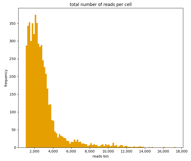
Finally it’s time to start exploring the loaded data. A usual first step is to examine the number of reads per cell. Cells with an unusual high or low number of reads may be artifacts and can be filtered out. We can generate a histogram of the total number of reads of cells with the command:

# These how's are supported: violin, boxplot and barplot.
ad.plotting.overall(exp, what='reads', how='histogram', bin_size=100)

Which will generate the plot:

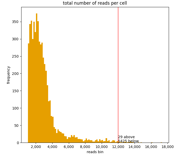
A vertical line can be included at any arbitrary threshold, for example to draw a red line at x=12,000 total reads by including the cut_off parameter:

ad.plotting.overall(exp, how='histogram', cut_off=12000)

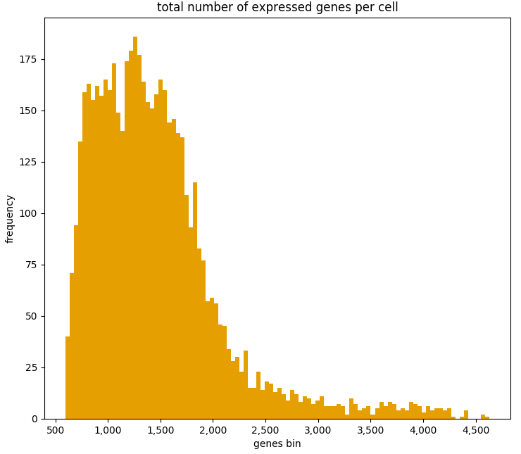
It can also be useful to examine the number of expressed genes per cell in order to detect any outliers:

ad.plotting.overall(exp, what='genes', how='histogram', bin_size=100)

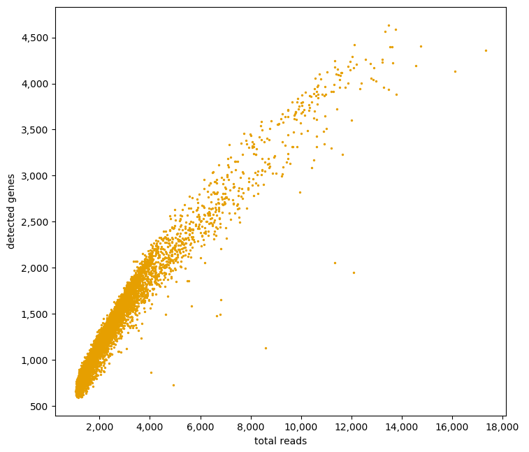
A third informative plot is to relate the number of detected genes with the total read depth into a scatter plot:

ad.plotting.overall_scatter(exp)

Detecting ERCC spikes

ERCC are known amounts of synthetic constructs added to RNA-seq libraries for quality control and normalization purposes [1]. Not all experiments use ERCC spikes, but many do. The ERCC “genes” are usually prefixed with ERCC- in the gene expression matrix. If ERCCs are present, then we need to let adobo know about them so that these spikes are not included in downstream analyses. adobo.preproc.find_ercc() is used to flag the ERCC spikes (stored in the ERCC column of adobo.data.dataset.meta_genes):

ad.preproc.find_ercc(exp, ercc_pattern='^ERCC[_-]\\S+$')

Detecting mitochondrial genes

Mitochondrial gene expression signals can serve to indirectly tell us how healthy the captured cells are. Dying and low quality cells tend to exhibit unusually high signal from these genes. One convenient function identifies mitochondrial genes in your data and adds the percent of mitochondrial gene expression to the cellular meta data. Often mitochondrial genes in the human and mouse genomes have gene symbols starting with the prefix mt-, but this might vary from species to species.

ad.preproc.find_mitochondrial_genes(exp, mito_pattern='^mt-')

Sometimes a regular expression is not possible and we can instead supply a list of gene IDs or symbols representing mitochondrial genes:

ad.preproc.find_mitochondrial_genes(exp, genes=['geneA','geneB','geneC'])

Data filtering

Applying simple filters

Simple filters refers to applying a strict minimum cutoff on the number of expressed genes per cell and the total read depth per cell. Simple filters are usually effective in removing low quality cells and uninformative genes. If your data come from Drop-seq, 10X, etc, requiring at least 1000 uniquely mapped reads per cell is often sufficient:

ad.preproc.simple_filter(exp, minreads=1000, minexpgenes=0.001)

Important

If your protocol is applying full-length mRNA sequencing, e.g. SMART-seq2, then your minreads threshold should be higher, for example 50000.

Note

adobo.preproc.simple_filter() also has a maxreads parameter, which can be used to remove cells with an upper read count limit (perhaps useful for limiting doublets). However, this parameter is not set by default.

It is also desirable to remove genes with an expression signal in very few cells; such genes may contribute more noise than information. The minexpgenes parameter can be used to control how genes are filtered out. If you wish to not remove any genes at all, simply set it to zero:

ad.preproc.simple_filter(exp, minreads=1000, minexpgenes=0)

Setting minexpgenes to a fraction indicates that at least that fraction of cells must express any gene. If minexpgenes is an integer it refers to the absolute number of cells that at minimum must express the gene for the gene not to be filtered out.

To reset all simple filters to original:

exp.reset_filters()

Dynamic detection of low quality cells

A more sophisticated approach to detection of low quality cells is to use the function adobo.preproc.find_low_quality_cells(), which uses Mahalanobis distance to identify bad cells from five quality metrics.

Important

find_low_quality_cells requires that there are ERCC spikes in your data.

The parameter rRNA_genes should either be a string containing the full path to a file on disk contaiing genes that are rRNA genes (the file should have one gene per line). rRNA_genes can also be a pandas.Series object with gene symbols.

ad.preproc.find_low_quality_cells(exp, rRNA_genes=rRNA)

Like all adobo functions, find_low_quality_cells modifies the passed object. However, find_low_quality_cells also returns a list of cells that are classified as low quality; to prevent such behavior simply assign the return to a variable:

low_q_cells = ad.preproc.find_low_quality_cells(exp, rRNA_genes=rRNA)

Imputation of dropouts

“Dropouts” are artifacts caused by the low amounts of mRNA in single cells, causing expressed genes to become undetected in the expression data. Droplet-based protocols tend to have a greater number of dropouts. Several statistical procedures have been developed to impute missing expression values. adobo implements the method introduced by Li et al [2]. The original paper describes the theory; briefly, model parameters are estimated using the Gamma distribution, then it uses Elastic net regularization to fit a linear model, which is used to predict expression values of genes with zero expression. adobo’s imputation function is adobo.preproc.impute():

ad.preproc.impute(exp, filtered=True, res=0.5, nworkers='auto', verbose=True)

The parameter filtered is used to indicate if imputation should run on the quality-filtered data or on the complete raw read count matrix (default is to run on the filtered). Parallelization is achieved using Python’s multiprocessing module. The parameter nworkers can be used to set the number of worker processes, which can be ‘auto’ to autodetect this (although due to Python’s Global Interpreter Lock the number of workers should not be higher than the number of physical cores). Imputed data are stored in adobo.data.dataset.imp_count_data. If you have a low number of cells (<1000), set the cluster resolution parameter to something low, for example res=0.1.

Note

Runtime varies depending on number of physical cores and size of the dataset. Typical runtime for a dataset consisting of ~1000 cells using 10 cores is 15 min.

Normalization

Normalization removes technical and sometimes experimental biases and is always necessary prior to analysis. Because a universal normalization scheme for scRNA-seq data is not available nor recommended, adobo supports several different procedures. The function adobo.normalize.norm() can be used to perform the following normalization methods:

standard

Performs a standard normalization by scaling with the total read depth per cell and then multiplying with a scaling factor.

rpkm

Normalizes read counts as Reads per kilo base per million mapped reads (RPKM) [3]. This method should be used if you want to adjust for gene length, such as in a full-length mRNA protocol. To use this procedure you must first prepare a file containing combined exon lengths for genes; the file should contain two columns, without a header, and columns separated by one space. The following columns must be present: (1) gene symbols and (2) the sum of exon lengths. The filename is set with the gene_lengths parameter, which can also take a vector.

fqn

Performs full quantile normalization [4]. FQN was a popular normalization scheme for microarray data. It is not very common in single cell analysis despite having been shown to perform well [5]. The present implementation does not handle ties well.

clr

Centered log ratio normalization. This normalization scheme was introduced in Seurat version 3.0 [6]. It is a simple normalization scheme and is an alternative to standard.

vsn

Variance stabilizing normaliztion based on a negative binomial regression model with regularized parameters. Introduced by [7] and represents a more sophisticated normalization approach. Appears to marginally improve resolution. Can be used if you have UMI counts.

All normalization schemes can be followed by log-transformation by setting log=True, which is default behavior. The log function can be set with the log_func parameter (default is numpy’s log2 ).

To perform a standard normalization followed by log-transformation, run:

ad.normalize.norm(exp, method='standard')
ad.normalize.norm(exp, method='clr')

The normalized data are stored in the attribute adobo.data.dataset.norm_data, which is a dictionary of dictionaries. If we run multiple normalizations they are all stored in the norm_data and we can use the name name parameter in adobo.normalize.norm() to give it a name (default name is the method). We can always call is_normalized() to determine if a dataset has been normalized:

>>> exp.is_normalized()
True

Note

If you have previously executed adobo.preproc.find_ercc(), ERCC spikes will be normalized too, and these can be found in adobo.data.dataset.norm_ercc.

If you want to normalize using imputed data, then set the use_imputed to True:

ad.normalize.norm(exp, use_imputed=True, method='standard')

Examining analysis history

Downstream analyses are performed on the data object. At any time it’s possible to examine what functions have been applied on data object by calling adobo.data.dataset.assays():

>>> exp.assays()
Number of mitochondrial genes found: 0
Number of ERCC spikes found: 92
Normalization method: <not performed yet>
Has HVG discovery been performed? No

When we run a function, it often generates results, which are stored in your data object. Specifically, results are stored in the norm_data dictionary. norm_data is where all analysis results are stored and it has a nested structure that can be displayed interactively by giving the name of the data object.

Detection of highly variable genes

Many algorithms used in scRNA-seq analysis perform better when used on a subset of measured genes [8]; the goal of the feature selection step is usually to extract a set of highly variable genes (HVG). adobo currently implements the following strategies for HVG discovery:

seurat

The function bins the genes according to average expression, then calculates dispersion for each bin as variance to mean ratio. Within each bin, Z-scores are calculated and returned. Z-scores are ranked and the top 1000 are selected. Input data should be normalized first. This strategy was introduced in Seruat [6], it is simple yet highly effective in identifying HVG.

brennecke

Implements the method described in [9]. brennecke estimates and fits technical noise using ERCC spikes (technical genes) by fitting a generalized linear model with a gamma function and identity link and the parameterization w=a_1+u+a0. It then uses the chi2 distribution to test the null hypothesis that the squared coefficient of variation does not exceed a certain minimum. False discovery rate (FDR)<0.10 is considered significant.

scran

scran fits a polynomial regression model to technical noise by modeling the variance versus mean gene expression relationship of ERCC spikes (the original method used local regression) [10]. It then decomposes the variance of the biological gene by subtracting the technical variance component and returning the biological variance component.

chen2016

This method uses linear regression, subsampling, polynomial fitting and gaussian maximum likelihood estimates to derive a set of HVG [11].

mm

Selection of HVG by modeling dropout rates using modified Michaelis-Menten kinetics [12]. This method calculates dropout rates and mean expression for every gene, then models these with the Michaelis-Menten equation (parameters are estimated with maximum likelihood optimization). The basis for using MM is because most dropouts are caused by failure of the enzyme reverse transcriptase, thus the dropout rate can be modelled with theory developed for enzyme reactions. This implementation works best for libraries sequenced to saturation (i.e. not Drop-seq).

Example:

ad.hvg.find_hvg(exp, method='seurat', ngenes=1000)

Dimensional reduction

These are techniques to reduce the number of dimensions under consideration.

Principal Component analysis (PCA)

PCA decomposition [13] of single cell data is for the most part necessary prior to clustering. The reason for this is because the graph construction benefits from a strong signal from each feature. PCA computation in adobo is performed by invoking adobo.dr.pca(). Scaling of the data should always be performed before PCA, and this is done by default (although it can be turned off by setting scale=False). Two approaches are available for PCA decomposition, and it should not matter much which one is used:

irlb

Computed via truncated singular value decomposition by implicitly restarted Lanczos bidiagonalization [14]. irlb may be better at handling very large single cell datasets and it is the default.

svd

The standard approach to PCA. Computed via singular value decomposition (svd). (More likely to raise MemoryError.)

Examples:

# 75 components are returned by default, may need to be adjusted depending on your dataset
ad.dr.pca(exp, method='irlb', ncomp=75)

# or...

ad.dr.pca(exp, method='svd', ncomp=75)

We can now examine the top contributing genes to each PCA component by producing a plot with adobo.plotting.pca_contributors().

To plot the top 10 contributing genes to the first five components:

ad.plotting.pca_contributors(exp, dim=[0,1,2,3,4], top=10)

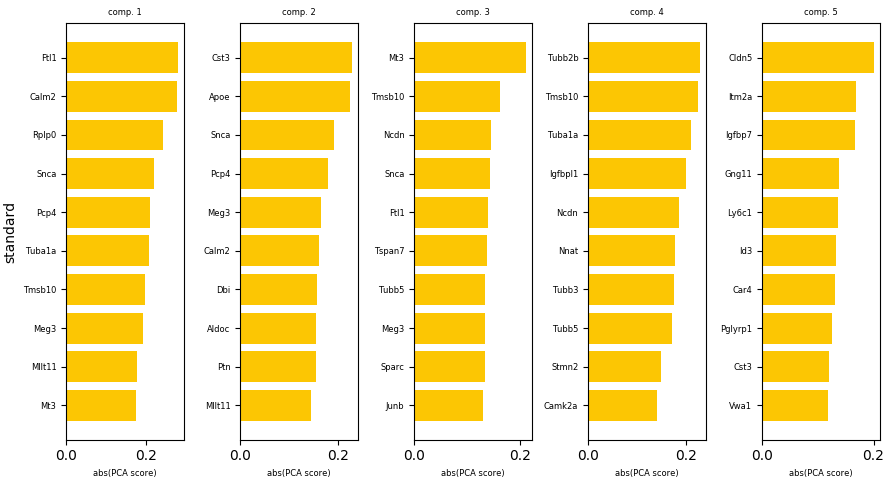
We can also write the output to a file instead of showing it on the screen:

ad.plotting.pca_contributors(exp, dim=[0,1,2,3,4], top=10, filename='top_pca_genes.pdf')

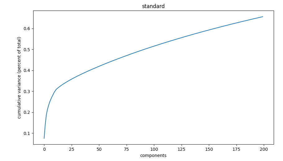
The default number of components, 75, is often sufficient. However, a more deterministic approach is to generate an elbow plot using adobo.plotting.pca_elbow():

ad.plotting.pca_elbow(exp)

t-Distributed Stochastic Neighbor Embedding (t-SNE)

t-SNE [15] is a non-linear dimensional reduction technique that optimizes for local distance. It is the de facto dimensional reduction technique used to visualize scRNA-seq data [16]. adobo uses the scikit-learn implementation [17]. The most important parameter is perplexity (related to number of nearest neighbors) and it can greatly influence how your plot looks like. Suggested values for perplexity lies between 5 and 50, and it is recommened to try higher values for datasets with more cells. Additional parameters (such as early_exaggeration, learning_rate, n_iter, and n_iter_without_progress) do not usually need to be specified but will be passed into sklearn.manifold.TSNE. By default adobo runs t-SNE on the PCA decomposition:

ad.dr.tsne(exp, perplexity=30, run_on_PCA=True, verbose=True)

The recommended approach is to run t-SNE on PCA components, but it can sometimes be informative to run it on your entire normalized expression matrix (this will take significantly longer time):

Note

t-SNE is non-deterministic. Different runs can give different results. To get a more reproducible t-SNE plot consider setting the seed parameter to any random integer, which will generate reproducible random numbers.

Uniform Manifold Approximation and Projection (UMAP)

UMAP [18] is also used frequently to visualize scRNA-seq data, and it may be better at preserving the global structure of the data:

ad.dr.umap(exp)

UMAP has a number of tunable parameters, for example n_epochs (try values between 100 to 2000).

Clustering

A crucial step in scRNA-seq analysis is to group cells into clusters. Complex datasets consisting of thousands of cells can be reduced to a small number of clusters, which tend to be easier to analyze and interpret.

Important

Clustering is performed in PCA space, therefore PCA components must have been calculated first using adobo.dr.pca().

In adobo, clustering can be performed with a single line of code:

# run leiden
ad.clustering.generate(exp, distance='euclidean', res=0.8, clust_alg='leiden')

# run louvain
ad.clustering.generate(exp, distance='euclidean', res=0.8, clust_alg='louvain')

# run walktrap
ad.clustering.generate(exp, distance='euclidean', clust_alg='walktrap')

The above command will run the necessary steps to cluster your single cell dataset; the cluster membership vector is stored in adobo.data.dataset.clusters, i.e. represented by an array with the same length as the number of cells after pre-processing. adobo’s default clustering algorithm first builds a Shared Nearest Neighbor graph [19] and then finds communities in this graph using the Leiden algorithm [20] (default). It may become necessary to change value of the res (resolution) parameter to find the optimal clustering outcome.

By default adobo.clustering.generate() will return a dict containing cluster sizes (number of cells), use retx=False to disable this behavior.

Other community detection algorithms are also supported via the igraph package:

• louvain [21]

• walktrap [22]

• spinglass [23]

• multilevel [21]

• infomap [24]

• label_prop (label propagation) [25]

• leading_eigenvector (Newman’s leading eigenvector method) [26]

Various parameters of the these algorithms can be changed in adobo.clustering.generate().

Note

spinglass does not scale well on large datasets [27].

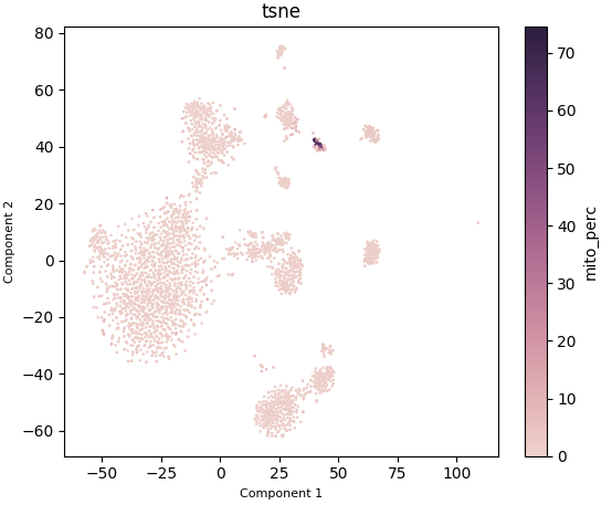
Clustering visualization

Visualization of cells in 2d space is performed with the function adobo.plotting.cell_viz(). Before running cell_viz, the appropriate reduction functions must have been invoked (t-SNE or UMAP; see above). cell_viz can plot custom meta data, gene expression, and clustering outcomes. Three parameters specified as tuples control what to plot:

clustering

Default is ‘leiden’.

metadata

Specify variable(s) listed as meta data in adobo.data.dataset.meta_cells (added via adobo.data.dataset.add_meta_data()).

genes

Specify any gene symbol(s).

The above parameters can be mixed and will in such cases generate one subplot for every specified variable. The ncols parameter can be used to set the number of columns in the plot (default is 2).

Examples:

# tsne
ad.plotting.cell_viz(exp, reduction='tsne', clustering='leiden', metadata='detected_genes')

# plots 'leiden' by default
ad.plotting.cell_viz(exp, reduction='umap')

Plotting mitochondrial gene expression:

ad.plotting.cell_viz(exp, reduction='tsne', meta_data='mito_perc', clustering=(), genes=())

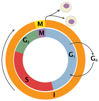
Cell cycle prediction

It is often useful to get an understanding of cell cycle states in a new data set, and it boils down to predicting one of three cell cycle states for every cell: G1, S and G2M. An extreme simplification of the cell cycle is shown below (figure from Wikipedia).

adobo contains a machine learning classifier based on the sklearn implementation of Stochastic Gradient Descent. The classifier is trained on mouse embryonic stem cells (n=288 cells) [28]. The original data can be retrieved from here. Cell cycle classification is performed by calling two functions:

# trains the classifier
clf, tr_features = ad.bio.cell_cycle_train()

# performs the actual classification of cells in your data
ad.bio.cell_cycle_predict(exp, clf, tr_features)

Classification is stored in the attribute adobo.data.dataset.meta_cells in a column cell_cycle. The current design does not support prediction scores, although this can easily be changed by changing the loss parameter.

We can visualize the results:

ad.plotting.cell_viz(exp, metadata='cell_cycle', clustering=(), genes=())

Important

Prediction is only valid on mouse data since the classifier is trained on mouse data. Make sure your gene expression contains Ensembl gene identifiers in one of the following two formats: ENSEMBL; GENESYMBOL_ENSEMBL.

Cell type prediction

Runs marker-based cell type prediction. The predictable unit is a cell cluster, meaning that cell clustering must have been performed before prediction is called. Cell type prediction works on mouse and human data. Gene symbols must be ued in your data (not Ensembl identifiers). If your data use Ensembl identifiers, the function adobo.preproc.symbol_switch() can be used to switch to gene symbols.

The min_cluster_size parameter specifies which clusters to ignore (i.e. clusters with fewer cells than this are ignored). Will run on all normalizations and clusterings as default (or specify which one with name and clustering).

ad.bio.cell_type_predict(exp, min_cluster_size=10, verbose=True)

The output is stored in the attribute adobo.data.dataset.norm_data.

Differential expression (DE)

DE analysis between is usually a key goal in the analysis workflow. In adobo, DE analysis can be performed between clusters or experimental groups (as defined by meta data). Currently, DE can be performed using linear models or Mann-Whitney U test (also called Wilcoxon rank-sum test). Linear models are significantly faster than performing individual hypothesis tests, but underlying assumptions may be violated and cause inflation of p-values. It is therefore sometimes preferred to use a non-parametric test, which albeit robust is substantially slower.

For linear models, significance is calculated from coefficients using t statistics.

To execute a LM-driven DE analysis:

ad.de.linear_model(exp)

The above command runs pairwise comparisons between all clusters.

We might prefer to use the Mann–Whitney U test:

# if nworkers is auto, the complete number of physical cores will be used
# logical cores will likely not result in speedup due to Python's thread safety
ad.de.wilcox(exp, nworkers='auto')

After running pairwise tests, a next typical goal is to join p-values so that each cluster receives a single list of marker genes. P-value merging can be achieved the following call:

ad.de.combine_tests(exp, method='fisher', mtc='bonferroni', retx=True, verbose=True)

The above generate a set of marker genes for every cluster using Fisher’s method.

Indices and tables

• Index

• Module Index

References

1

Lichun Jiang, Felix Schlesinger, Carrie A. Davis, Yu Zhang, Renhua Li, Marc Salit, Thomas R. Gingeras, and Brian Oliver. Synthetic spike-in standards for RNA-seq experiments. Genome Research, 21(9):1543–1551, September 2011. doi:10.1101/gr.121095.111.

2

Wei Vivian Li and Jingyi Jessica Li. An accurate and robust imputation method scImpute for single-cell RNA-seq data. Nature Communications, 9(1):997, March 2018. doi:10.1038/s41467-018-03405-7.

3

Ana Conesa, Pedro Madrigal, Sonia Tarazona, David Gomez-Cabrero, Alejandra Cervera, Andrew McPherson, Michał Wojciech Szcześniak, Daniel J. Gaffney, Laura L. Elo, Xuegong Zhang, and Ali Mortazavi. A survey of best practices for RNA-seq data analysis. Genome Biology, 17(1):13, January 2016. doi:10.1186/s13059-016-0881-8.

4

B.M. Bolstad, R.A Irizarry, M. Åstrand, and T.P. Speed. A comparison of normalization methods for high density oligonucleotide array data based on variance and bias. Bioinformatics, 19(2):185–193, 01 2003. doi:10.1093/bioinformatics/19.2.185.

5

Michael B. Cole, Davide Risso, Allon Wagner, David DeTomaso, John Ngai, Elizabeth Purdom, Sandrine Dudoit, and Nir Yosef. Performance assessment and selection of normalization procedures for single-cell rna-seq. bioRxiv, 2018. doi:10.1101/235382.

6(1,2)

Tim Stuart, Andrew Butler, Paul Hoffman, Christoph Hafemeister, Efthymia Papalexi, William M Mauck III, Marlon Stoeckius, Peter Smibert, and Rahul Satija. Comprehensive integration of single cell data. bioRxiv, 2018. doi:10.1101/460147.

7

Christoph Hafemeister and Rahul Satija. Normalization and variance stabilization of single-cell rna-seq data using regularized negative binomial regression. bioRxiv, 2019. doi:10.1101/576827.

8

Shun H Yip, Pak Chung Sham, and Junwen Wang. Evaluation of tools for highly variable gene discovery from single-cell RNA-seq data. Briefings in Bioinformatics, 02 2018. doi:10.1093/bib/bby011.

9

Philip Brennecke, Simon Anders, Jong Kyoung Kim, Aleksandra A Kołodziejczyk, Xiuwei Zhang, Valentina Proserpio, Bianka Baying, Vladimir Benes, Sarah A Teichmann, John C Marioni, and Marcus G Heisler. Accounting for technical noise in single-cell RNA-seq experiments. Nature Methods, 10:1093, September 2013. URL: https://doi.org/10.1038/nmeth.2645.

10

Aaron T. L. Lun, Davis J. McCarthy, and John C. Marioni. A step-by-step workflow for low-level analysis of single-cell RNA-seq data with Bioconductor. F1000Research, 5:2122, 2016. doi:10.12688/f1000research.9501.2.

11

Hung-I Harry Chen, Yufang Jin, Yufei Huang, and Yidong Chen. Detection of high variability in gene expression from single-cell RNA-seq profiling. BMC Genomics, 17(7):508, August 2016. doi:10.1186/s12864-016-2897-6.

12

Tallulah S Andrews and Martin Hemberg. M3Drop: dropout-based feature selection for scRNASeq. Bioinformatics, 35(16):2865–2867, 12 2018. doi:10.1093/bioinformatics/bty1044.

13

Hervé Abdi and Lynne J. Williams. Principal component analysis. Wiley Interdisciplinary Reviews: Computational Statistics, 2(4):433–459, 2010. doi:10.1002/wics.101.

14

James Baglama and Lothar Reichel. Augmented implicitly restarted lanczos bidiagonalization methods. SIAM J. Sci. Comput., 27(1):19–42, July 2005. doi:10.1137/04060593X.

15

Laurens van der Maaten and Geoffrey Hinton. Visualizing data using t-SNE. Journal of Machine Learning Research, 9:2579–2605, 2008.

16

Dmitry Kobak and Philipp Berens. The art of using t-sne for single-cell transcriptomics. bioRxiv, 2019. doi:10.1101/453449.

17

F. Pedregosa, G. Varoquaux, A. Gramfort, V. Michel, B. Thirion, O. Grisel, M. Blondel, P. Prettenhofer, R. Weiss, V. Dubourg, J. Vanderplas, A. Passos, D. Cournapeau, M. Brucher, M. Perrot, and E. Duchesnay. Scikit-learn: machine learning in Python. Journal of Machine Learning Research, 12:2825–2830, 2011.

18

Leland McInnes, John Healy, and James Melville. UMAP: Uniform Manifold Approximation and Projection for Dimension Reduction. arXiv e-prints, pages arXiv:1802.03426, Feb 2018. arXiv:1802.03426.

19

Levent Ertöz, Michael Steinbach, and Vipin Kumar. Finding clusters of different sizes, shapes, and densities in noisy, high dimensional data. In in Proceedings of Second SIAM International Conference on Data Mining. 2003.

20

V. A. Traag, L. Waltman, and N. J. van Eck. From Louvain to Leiden: guaranteeing well-connected communities. Scientific Reports, 9(1):5233, March 2019. doi:10.1038/s41598-019-41695-z.

21(1,2)

Vincent D Blondel, Jean-Loup Guillaume, Renaud Lambiotte, and Etienne Lefebvre. Fast unfolding of communities in large networks. Journal of Statistical Mechanics: Theory and Experiment, 2008(10):P10008, Oct 2008. URL: http://dx.doi.org/10.1088/1742-5468/2008/10/P10008, doi:10.1088/1742-5468/2008/10/p10008.

22

Pascal Pons and Matthieu Latapy. Computing Communities in Large Networks Using Random Walks. Journal of Graph Algorithms and Applications, 2006.

23

Joerg Reichardt and Stefan Bornholdt. Statistical mechanics of community detection. Physical Review E, 74:016110, 2006.

24

Martin Rosvall and Carl T. Bergstrom. Maps of random walks on complex networks reveal community structure. Proceedings of the National Academy of Sciences, 105(4):1118–1123, 2008. doi:10.1073/pnas.0706851105.

25

Usha Nandini Raghavan, Réka Albert, and Soundar Kumara. Near linear time algorithm to detect community structures in large-scale networks. Phys. Rev. E, 76:036106, Sep 2007. doi:10.1103/PhysRevE.76.036106.

26

M. E. J. Newman. Finding community structure in networks using the eigenvectors of matrices. Phys. Rev. E, 74:036104, Sep 2006. doi:10.1103/PhysRevE.74.036104.

27

Zhao Yang, René Algesheimer, and Claudio J. Tessone. A Comparative Analysis of Community Detection Algorithms on Artificial Networks. Scientific Reports, 6:30750, August 2016. URL: https://doi.org/10.1038/srep30750.

28

Florian Buettner, Kedar N Natarajan, F Paolo Casale, Valentina Proserpio, Antonio Scialdone, Fabian J Theis, Sarah A Teichmann, John C Marioni, and Oliver Stegle. Computational analysis of cell-to-cell heterogeneity in single-cell RNA-sequencing data reveals hidden subpopulations of cells. Nature Biotechnology, 33:155, January 2015.